Knot theory

Knots (links) are embeddings of the circle (some finite number of circles) into the 3-sphere, modulo ambient isotopy. Knot theory is thus the study of the essentially different ways we can embed a circle into a 3-sphere—a kind of deformation theory for such maps, if you will. From this perspective, it is perhaps not too surprising that knot theory has developed connections to many areas of pure and applied mathematics.

For example, knot complements and Dehn surgery are important sources of examples for 3-manifolds. Knot complements are intimately related to knots themselves, by the Gordon-Luecke theorem; Dehn surgery not only has the virtue of being explicitly computable, it is also a fairly generic source of 3-manifolds, by the Lickorish-Wallace theorem.

Or, for example, knot theory shows up in physics in various ways. Indeed, knot theory and physics tangled from fairly early on: most prominently, Lord Kelvin’s theory of “vortex atoms” posited that atoms can be modeled as knots of aether. While this turned out to be wrong from a physical standpoint, it did inspire Tait to start classifying knots and spur the mathematical development of knot theory; and it may yet find a spiritual successor in the “anyons” of topological quantum computing.

Yet another early connection can be seen in the linking number, one of the first knot (or link) invariants, which Gauss came up in his study of a question from electrodynamics: how much work is done on a magnetic pole moving along a closed loop in the presence of a loop of current? Using the Ampere and Biot-Savart law, he found the answer could be described in terms of how many times one of these loops winds around the other, or in other words the linking number of the two loops (see e.g. pp. 2-4 here.)

Knot invariants

More generally, knot (or link) invariants are mathematical objects—numbers, polynomials, homology groups, whatever have you—attached to knots (or links—I’ll stop writing this, but you should imagine inserted after each instance of “knot” below.) Equivalent (i.e. ambient-isotopic) knots should be assigned the same value—hence the name “invariant”—although certain pairs of non-equivalent knots may also be assigned equal values.

These are useful, primarily, for distinguishing knots—for providing a verifiable certificate that two knots are indeed inequivalent, as it were.

It is straightforward enough, in principle, to prove that two knots are equivalent: one simply exhibits an ambient isotopy taking one to the other. Indeed, this ambient isotopy can always be described within an explicitly-described standard combinatorial model—using a class of standard local “moves”, the Reidemeister moves, on knot diagrams, i.e. projections of the knot to a plane, decorated with additional information about which strand crosses “over” the other at each double point.

(Completely tangential aside: knot diagrams can be an endless source of combinatorial fun—see e.g. this REU paper on games on shadows of knots.)

It is rather harder to prove that two knots are inequivalent this way: failure to exhibit a suitable sequence of Reidemeister moves doesn’t prove that an ambient isotopy can’t exist—perhaps with more ingenuity one could in fact find the requisite Reidemeister moves? Hence the utility of knot invariants: if we can show that two knots take on different values for a certain knot invariant, that definitively shows that they are inequivalent.

Some examples of knot invariants include the crossing number—which can be defined as the minimum number of crossings (double points) which any knot diagram of a given knot must have—, the unknotting number—which can be defined as the least number of times one needs to pass a knot through itself (or, equivalently, the least number of crossings that need to be switched) to get to an unknot—, and the Seifert genus—the minimal genus of any connected oriented surface whose boundary is the knot.

These invariants are intuitive and natural measures of the “complexity” of a knot, but are notoriously hard to compute and study. For instance, it is conjectured, but still not known, that the crossing number is additive under taking connect-sums, and it took a surprising amount of work (an Inventiones paper!) to show that composite knots have unknotting number at least 2. In some sense, an understanding of these invariants can be seen as a primary aim, rather than a tool, of knot theory.

More computable, but in some ways less intuitive and more mysterious, are invariants of a more algebraic nature: things such as the signature or Arf invariant coming from naturally-associated quadratic forms, or various knot polynomials which package this and other knot data into their coefficients. The theory behind and extending from these knot polynomials, in particular has driven much of modern knot theory, and we touch on some of these developments below.

The turn to combinatorics (and algebra)

Starting with Conway’s work on the Alexander polynomial in the 1960s, it has been realized that many of these polynomials can be defined and computed combinatorially, using skein relations; building on this, and introducing language and ideas from statistical mechanics, Kauffman formulated state-sum models for computing the Alexander and Jones polynomials in the 1980s.

This was not the first time physics had popped up here, either: models from statistical mechanics motivated the von Neumann algebras and braid representations which were originally used to define the Jones polynomial. This was in many ways a pivotal development in the theory: to borrow The Unapologetic Mathematician’s words:

Jones was studying a certain kind of algebra when he realized that the defining relations for these algebras were very much like those of the braid groups. In fact, he was quickly able to use this similarity to assign a Laurent polynomial … to every knot diagram that didn’t change when two diagrams differed by a Reidemeister move. That is, it was a new invariant of knots.

The Jones polynomial came out of nowhere, from the perspective of the day’s knot theorists. And it set the whole field on its ear. From my perspective looking back, there’s a huge schism in knot theory between those who primarily study the geometry and the “classical topology” of the situation and those who primarily study the algebra, combinatorics, and the rising field of “quantum topology”. To be sure there are bridges between the two … But the upshot was that the Jones polynomial showed a whole new way of looking at knots and invariants.

Extending the skein relation approach to build invariants on a larger class of knots with singular points leads us to the theory of the much more powerful, and possibly fundamental finite-type (Vassiliev) invariants, which has subsequently been studied using such tools as chord diagrams and the Kontsevich integral.

Knot homology theories

Another, related direction in which knot polynomials have taken off is towards homological algebra, in a development sometimes described as “categorification”. Categorifying a knot polynomial involves building a homology whose Euler characteristic—in an appropriate sense, involving some sort of alternating sum of data from the homology groups—recovers the knot polynomial.

The homology groups of a topological space contain all the information carried by the Euler characteristic, and then some; in some sense, they are the more fundamental invariant, of which the Euler characteristic is just a “decategorified shadow”. Similarly, a knot homology theory should be, in principle at least, more powerful and fundamental than the polynomial it categorifies .

The two main (flavors of) knot homology are Khovanov homology and knot Floer homology. Khovanov homology, developed in the late 1990s by Mikhail Khovanov, is related to ideas in representation theory, and categorifies the Jones polynomial. Knot Floer homology, developed by Ozsváth and Szabó and independently by Rasmussen, both in the early 2000s, is based off Heegaard Floer theory, “a symplectic geometric replacement for gauge theory”, and categorifies the Alexander polynomial.

There are connections between these homology theories and Lie algebras, symplectic geometry, 3- and 4-dimensional topology, physics, and so on, about which I am entirely ignorant at the moment …

Quantum things (also, strings)

Quantum mechanics has already made a brief cameo above. Indeed, as hinted but not spelt out above, many pieces of mathematics which appear in quantum mechanics and related physical theories can be leveraged to create knot invariants—e.g. the Jones polynomial can be recovered from Chern-Simons theory, and the Kontsevich integral is inspired by perturbative Chern-Simons theory.

The connections run much deeper—it appears that knots and braids provide, or are an integral part of, some of the most compelling mathematical models for quantum phenomena, and even make aspects of their appearance felt in string theory. Now, as before, knot theory remains intertwined with physics, although now mediated through the elaborate structure of representation theory in its various guises.

Articles

The Eskin-Mirzakhani-Mohammadi Magic Wand

Structure of orbits: a geometric Ratner’s theorem?

The ergodicity of the $\mathrm{SL}(2,\mathbb{R})$ action on the moduli space $\mathcal{H}$ of translation surfaces (= moduli space of Abelian differentials, under the identification we made earlier) allows us to understand generic orbits, but not of arbitrary orbits. In particular, for example, a family of flat surfaces correspond to a fixed rational polygonal billiard forms a positive-codimension subspace, about which ergodicity allows us to say nothing.

There are, however, results in dynamics / ergodic theory which classify not just almost all, but all orbits, the prototypical example being Ratner’s Theorem(s) on unipotent flows:

Theorem/s (Ratner) Let G be a connected Lie group and U be a connected subgroup generated by unipotents. Then

for any lattice $\Gamma \subset G$ and any $x \in G / \Gamma$ , the closure of the orbit $Ux \in G / \Lambda$ is an orbit of a closed algebraic subgroup of G.
every ergodic invariant probability measure is homogeneous;
every unipotent orbit is equidistributed in its closure.

A basic example is given by a horocycle flow on a hyperbolic manifold. These are ergodic, and so we know that almost every orbit is dense; but Ratner’s theorem tells us that in fact we have a strict dichotomy: every orbit is either closed or dense.

The hope here is for a similar result: one precise formulation of this is the following

Conjecture (“Magic Wand”) The closure of a $\mathrm{SL}(2,\mathbb{R})$ -orbit of any flat surface is a complex-algebraic suborbifold. (By a theorem of Kontsevich, any $\mathrm{SL}(2,\mathbb{R})$ -invariant complex suborbifold is represented by an affine subspace in cohomological period coordinates.)

Aspects of Teichmüller theory

Recall that we have identified $\mathcal{H}$ as a space of pairs (complex structure, holomorphic 1-form). Recalling some of the plumbings of Teichmüller theory, we consider also the space of pairs (complex structure, holomorphic quadratic differential), and identify it with the cotangent bundle to the moduli space $\mathcal{M}$ of complex structures. $\mathcal{H}$ can be identified with a subspace of $\mathcal{Q}$ consisting of those quadratic differentials which can be represented as global squares of holomorphic 1-forms.

This subspace may be considered as a “unit cotangent bundle”, being invariant under the Teichmüller geodesic flow (i.e. the diagonal subgroup action induced by the $\mathrm{SL}(2,\mathbb{R})$ action on $\mathcal{H}$ .)

We may check that $\mathrm{SL}(2,\mathbb{R})$ orbits in (the image of) $\mathcal{H}$ in $\mathcal{Q}$ descend to isometric maps of $\mathrm{SL}(2,\mathbb{R}) / \mathrm{SO}(2) \cong \mathbb{H}^2$ to $\mathcal{M}$ —i.e. the projections of these orbits are Teichmüller discs, also known as complex geodesics.

Complex geodesics may be described more directly in terms of the language of flat surfaces as follows: recall $\mathrm{SL}(2,\mathbb{R})$ orbits in $\mathcal{H}$ correspond to translation surfaces with a distinguished direction, encoded by the holomorphic 1-form; the $\mathrm{SL}(2,\mathbb{R})$ action changes the translation structure, i.e. the fundamental polygon, but not the affine structure, i.e. the resulting translation surface. Then we obtain a complex geodesic by forgetting the 1-form, i.e. forgetting the distinguished direction.

The classification of orbits is then closely related to the classification of these complex geodesics, which allows us to potentially use (even more) language and tools from Teichmüller theory.

“Revolution in genus 2”

Kontsevich-Zorich classified strata of the moduli space using spin structures and hyperellipticity. In genus 2, the two stratum $\mathcal{H}(2)$ and $\mathcal{H}(1,1)$ are each connected and consist entirely of hyperelliptic surfaces.

Smilie proved that closed $latex\mathrm{SL}(2,\mathbb{R})$-orbits—orbits of flat surfaces which are in some sense exceptionally symmetric—correspond exactly to orbits of Veech surfaces (see first post on polygonal billiards for a description of Veech surfaces.) The identification of closed orbits thus reduces to (or, at any rate, is equivalent to) the classification of Veech surfaces, about which some things, but not very many, are known.

McMullen proved that there is (up to ramified coverings) only one Veech surface in the stratum $\mathcal{H}(1,1)$ , given by the regular decagon with identified opposite sides.

Calta and McMullen, using different methods, described all Veech surfaces in $\mathcal{H}(2)$ —there is a countable family even up to ramified coverings—and gave efficient algorithms to recognize and classify these.

They also describe invariant submanifolds of intermediate dimension—intermediate between the full stratum and but larger than single closed orbits.

Finally, McMullen shows, using all of this, plus more subtle tools, that our “magic wand” conjecture is true in genus 2; the classification is in fact rather more precise, and he also obtains results about invariant measures in the spirit of Ratner’s theorems.

Eskin-Mirzakhani-Mohammadi’s magic wand

Mirzakhani and collaborators (Eskin and Mohammadi), together with Filip, in spectacular (relatively) recent work, proved the “magic wand” conjecture, plus measure rigidity results, for all genera.

The measure rigidity result of Eskin-Mirzakhani states that any ergodic P-invariant measure (where P is a maximal parabolic subgroup, e.g. the Borel subgroup) is in fact a Lebesgue class measure on a manifold cut out by linear equations, and must be $\mathrm{SL}(2,\mathbb{R})$ -invariant. This uses considerable machinery from ergodic theory: “almost 100 pages of delicate” entropy arguments, plus ideas of Benoist-Quint.

The theorem of Eskin-Mirzakhani-Mohammadi then builds on this to state that the $\mathrm{SL}(2,\mathbb{R})$ -orbit closure of a translation surface is always a manifold. Moreover, the manifolds that occur are locally defined by linear equations in period coordinates, with real coefficients and zero constant term.

The proof proceeds, given the measure rigidity result, by constructing a P-invariant measure on every P-orbit closure. Here the use of P, as opposed to $\mathrm{SL}(2,\mathbb{R})$ , is crucial—the former is amenable whereas the latter is not, and this allows us to use averaging methods in our construction.

(Filip’s result is needed to go from analyticity, which Eskin-Mirzakhani-Mohammadi actually gives us, to algebraicity.)

Where can the magic wand take us?

These results allow us to say things about specific families of translation surfaces—e.g. a rational billiard table, whose orbit under the $\mathrm{SL}(2,\mathbb{R})$ -action forms a high-codimension family in $\mathcal{H}$ —rather than just “almost all” translation surfaces

Thus, for instance, we can prove quadratic asymptotics (exact, not just lower and upper bounds as was previously the case) for the number of generalized diagonals, etc. in polygonal billiards.

There are many other instances where some problem may be naturally (re)formulated in terms of translation surfaces coming from polygonal billiards; then the magic wand implies additional structure on a relevant family of translation surfaces, which yields insight into the original problem. Below we outline two concrete examples of this:

The illumination problem

Given a room, how many light-bulbs are required to light it? Or, to abstract the problem a little: given a polygonal domain P (or really any planar domain, but let’s stick to polygons for now) and a point $x \in P$ , which points in P can (or cannot) be reached by billiard trajectories through x? A point y which can be reached from x is said to be illuminated from x.

Billiard trajectories very much resemble light-ray trajectories (at least locally)—indeed the word “optical” appeared in our description of billiard systems—and so it should be no surprise that the study of billiard systems and hence of translation surfaces yields insight into this and related problems. Indeed, as this wonderfully-named paper notes, the illumination problem “elementary properties which can be fruitfully studied using the dynamical behavior of the $\mathrm{SL}(2,\mathbb{R})$ -action on the moduli space of translation surfaces.”

Using the magic wand theorem, and that the geometric properties considered in the illumination problem produce closed sets of the moduli space $\mathcal{H}$ , Lelièvre-Monteil-Weiss have proved that, for any P and any $x \in P$ , there are finitely many $y \in P$ which are not illuminated from x.

The wind-tree model

The wind-tree model was originally formulated by statistical physicists Paul and Tatiana Ehrenfest as a model for a Lorenz gas: in this model, particles (the “wind”) travel in straight-line trajectories in the plane $\mathbb{R}^2$ , reflecting off rectangular obstacles (“trees”) placed along a $\mathbb{Z}^2$ lattice in a billiards-like fashion. One can also describe it, precisely, as billiards in the plane with these rectangles removed.

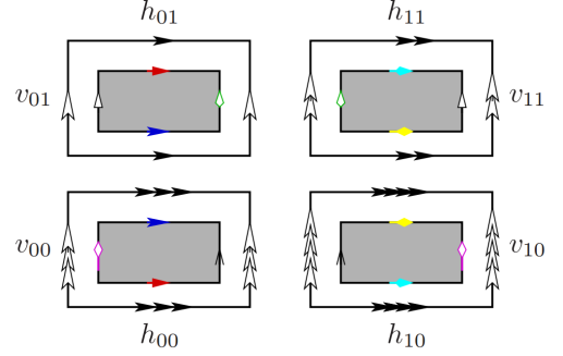
One can form a translation surface by restricting to some suitable subset of the plane and obstacles, and gluing the sides together: (figure taken from the also wonderfully-named “Cries and whispers in wind-tree forests“)

fig5

The result is a genus-5 flat surface in the stratum $\mathcal{H}(2^4)$ .

One can then describe the behavior of the trajectories in terms of properties of the translation surface, e.g. Delecroix-Hubert-Lelièvre have computed the diffusion of divergent trajectories, for rectangular obstacles of any size, in terms of the Lyapunov exponents of a natural dynamical system (the Kontsevich-Zorich cocycle) on a certain stratum of genus-5 translation surfaces—not the one specified above, but a quotient thereof.

References

Alex Wright’s article describes Eskin-Mirzakhani-Mohammadi result, the context for it, as well as applications and connections to nearby areas.

Articles

Translation surfaces and friends

Recall that we earlier defined translation surfaces as maximal atlases of coordinate charts into the Euclidean plane $\mathbb{R}^2$ , with finitely many cone singularities and where the transition maps between coordinate charts are translations in $\mathbb{R}^2$ .

Recall that we were led to this notion starting from polygonal billiards, but not every translation surface, generally defined, comes from a rational polygonal billiard.

Enter Riemann surfaces and moduli spaces

A translation surface may also be thought of as a Riemann surface, together with an associated holomorphic 1-form—a continuous choice of specified direction (“up”) at every point; such a pair of structures canonically defines a (singular) flat structure on the surface, with a distinguished vertical direction.

To wit: we take the holomorphic 1-form $\omega$ to be (locally) our dz. Since $\omega$ is holomorphic, its zeroes are isolated: a zero of degree d corresponds exactly to a conical singularity with cone angle $2\pi(d+1)$ . Where $\omega$ is not zero, it is represented (locally) by dz, whence we obtain a complex coordinate z, which in turn specifies (locally) a Euclidean structure. Since dz is globally well-defined on our translation surface, the resulting flat structure is also well-defined, away from the conical singularities.

Conversely, given a flat structure with conical singularities $P_1, \dots, P_n$ , and a specified direction, consider a fundamental polygon $P_1P_2 \cdots P_n$ embedded (anywhere, but with orientation dictated by the specified direction) in the complex plane. The fundamental polygon inherits a natural complex coordinate z. This does not descend to the translation surface, but since the identification maps are all of the form $z \mapsto z + \zeta$ where $\zeta \in \mathbb{C}$ is a constant (for each identification map), the holomorphic 1-form dz does, and we obtain a holomorphic 1-form $\omega$ on our translation surface. $\omega$ is zero exactly at the conical singularities, with cone angle being related to degree as above.

The Riemann surface perspective emphasizes more clearly the presence of a moduli space of translation surfaces (on for a fixed genus g), which we presently define as a space of pairs $(X, \omega)$ , where X denotes a Riemann surface structure, and $\omega$ a choice of holomorphic 1-form, modulo some natural equivalence relation. The 1-form specifies a distinguished direction—so there is a well-defined notion of “north” on the surface. Two such pairs $(X_1, \omega_1)$ and $(X_2, \omega_2)$ are considered equivalent if there is a conformal map from $X_1$ to $X_2$ which takes (specified) zeroes of $\omega_1$ to (specified) zeroes of $\omega_2$ .

The moduli space is divided into distinct strata $\mathcal{H}(d_1, \dots, d_m)$ , consisting of forms with zeroes of degree $d_1, \dots, d_m$ with $d_1 + \dots + d_m = 2g-2$ . This last identity follows from the formula for the sum of degrees of zeroes of a holomorphic 1-form on a Riemann surface of genus g, and can be interpreted as a Gauss-Bonnet formula for the singular flat metric.

There is a $\mathrm{SL}_2\mathbb{R}$ action on this moduli space (or, really, on each stratum) which is most easily described back in the framework of flat geometry: given any pair $(X,\omega)$ , build the corresponding flat polygon (with distinguished vertical direction.) Elements of $\mathrm{SL}_2\mathbb{R}$ act (linearly) on these flat polygons, thought of as being embedded in the Euclidean plane, with (say) some vertex at the origin. This action preserves parallelisms between edges; and hence is (induces) an action on the corresponding flat surfaces.

fig15

(figure from the Zorich survey—the $\mathrm{SL}(2,\mathbb{R})$ action, depicted on the left, changes the affine structure but not the translation structure; the “cut-and-paste” on the right changes the translation structure, but not the affine structure.)

We can study the dynamics of this action, and this turns out to be surprisingly (or perhaps not surprisingly—or maybe that is only with the benefit of giant-assisted hindsight) rich …

(There were already hints of this in the last post, when we talked about “changing the translation structure while preserving the affine structure” and how Masur used this idea to prove his theorem on counting closed geodesics.)

Counting closed geodesics and saddle connections

As previously noted in the slightly more restricted context of rational polygonal billiards, directional flow on a flat surface is uniquely ergodic in almost every direction.

This is most transparently seen in the case of a torus: geodesics with rational slopes are closed, while those with irrational slopes are equidistributed. Geodesics on flat surfaces of higher genera exhibit certain similiarities: the closed geodesics also appear in parallel families, although in higher genera these do not fill the whole surface, but only flat cylinders with conical singularities on the boundary.

Related to closed geodesic are saddle connections, which are geodesic segments joining two conical singularities (which may coincide), with no conical points in their interior. On a flat torus there are no conical singularities, and so any closed loop can be tightened to a closed geodesic; on a more general flat surface, this tightening process can produce either a closed geodesic, or—if at some point in the process we hit one of the singularities on the surface, which, as one might imagine, is the more generic case—a union of saddle connections.

Masur and Eskin have found quadratic asymptotics, as a function of length, for the number of [cylindrical families of] closed geodesics—this was discussed more in the previous post—and the number of saddle connections. The constants which appear in these asymptotics are called the Siegel-Veech constants. There are also (somewhat surprising) quadratic asymptotics for multiple cylindrical families in the same parallel direction.

These results are interesting in their own right—on a [rational] billiard table, for instance, generalized diagonals (trajectories joining two of the corners, possibly after reflections) unfold to saddle connections and periodic trajectories unfold to closed regular geodesics—but are also useful for at least two other reasons:

One, degeneration of “configurations” of parallel saddle connections or closed geodesics leads us into cusped regions in the boundary of (strata in the) moduli space, and so a description of such configurations gives us a description of the cusps of our strata. Local considerations involving short / degenerating saddle connections also lead us to relations between and structural results about the strata, which can be described more carefully / analytically in the language of Abelian differentials.

Two, configurations of saddle connections and closed geodesics are also useful as invariants of $\mathrm{SL}(2,\mathbb{R})$ orbits—something that we will refer back to below.

Volume of moduli space

We remark that this last counting problem can be related to computations of volumes of the moduli space, via the observation that the Siegel-Veech constants can be obtained as a limit of the form $\lim_{\epsilon \to 0} \frac{1}{\pi \epsilon^2} \frac{\mathrm{Vol}(\epsilon\mbox{-neighborhood of cusp }\mathcal{C})}{\mathrm{Vol} \mathcal{H}_1^\circ(d_1, \dots, d_n)}$ where $\mathcal{C}$ is a specified configuration of saddle connections or closed geodesics.

Athreya-Eskin-Zorich used this idea to obtain explicit formulas (conjectured by Kontsevich based on experimental evidence) for the volumes of strata in genus 0, by counting generalized diagonals and periodic trajectories on right-angled billiards. In general, of course, the relation between the two problems can be exploited in both directions: results on volumes of strata can also be used to obtain results on the counts of saddle connections / closed geodesics.

There are a number of alternative strategies for finding these volumes; the following is so far the most general:

The general idea is to simply use asymptotics for counts of integer lattice points, where the lattice is defined in terms of cohomological period coordinates. We can count the number of such points in a sphere or hyperboloid (which is the unit sphere for an indefinite quadratic form of suitable signature) to estimate its volume, and take a derivative to estimate the volume of the boundary hypersurface.

Integer lattice points may be thought of, geometrically, as flat surfaces tiled by square flat tori, and combinatorial geometric methods may be used to count these: in the simplest cases we can count directly; slightly more generally we can consider the graph with conical points as vertices and horizontal saddle connections as edges, leading to the notions of ribbon graphs and separatrix diagrams.

In the most general case we turn, following an idea of Eskin-Okounkov, to representation theory: suppose there are N squares; label them, and consider the permutation $\pi$ on [N] which sends j to the square $\pi(j)$ which we get to by starting at j and moving left, up, right, and down in turn. For the generic square j, $\pi$ fixes j, but near the conical points it acts non-trivially, and indeed it is a product of m cycles of lengths $(d_1+1), \dots, (d_m+1)$ .

It then suffices to count the number of permutations of N with such a property … except there is a nontrivial correction needed to pick out only those permutations which correspond to connected square-tiled surfaces. Eskin-Okounkov-Pandharipande pushed through this strategy to obtain explicit quantitative results, with a strong arithmetic flavor. These results may be made explicit, although there is considerable computational work involved; by comparison, other approaches such as the work of Athreya-Eskin-Zorich referred to above can produce simpler formulas in special cases.

Applications

We have described above and previously how translation surfaces are related to (rational) polygonal billiards, and how the former provide a powerful framework for the study of the latter. Here (and in a subsequent post) we present a number of other applications:

Electron transport

S. P. Novikov suggested the following as a mathematical formulation of electron transport in metals: consider a periodic surface $\widetilde{M^2} \subset \mathbb{R}^3$ ; an affine plane in $\mathbb{R}^3$ intersects this in some union of closed and unbounded intervals. Question: how does an unbounded component propagate in $\mathbb{R}^3$ (as we move the affine plane in some continuous fashion?)

After we quotient by the period lattice (taken to be $\mathbb{Z}^3$ ), we are looking at plane sections of the quotient surface $M^2 \subset \mathbb{T}^3$ . Our original intersection can be viewed as level curves of a linear function $f(x,y,z) = ax + by + cz$ restricted to $\widetilde{M^2}$ , but this does not push down to the quotient; instead, we consider the codimension-one foliation of $M^2$ defined by the closed 1-form $df = a\,dx + b\,dy + c\,dz$ .

Our question can then be reformulated as follows: what do lifts of leaves of this foliation on $M^2 \subset \mathbb{T}^3$ look like upstairs, in $\widetilde{M^2} \subset \mathbb{R}^3$ ?

Closed 1-forms on surfaces can be straightened to geodesic foliations in appropriate flat metrics iff any cycle formed from a union of closed paths following a sequence of saddle connections is homologically non-trivial. The surfaces and 1-forms obtained from Novikov’s problem can be modified (decomposed and surgered) to satisfy this criterion, and after these reductions we are left exactly in the world of flat structures with closed 1-forms on them, i.e. translation surfaces.

Invisibility

In a subsequent post we describe the illumination problem; a related problem concerns invisibility—more precisely: whether a body with mirror surfaces can be “invisible” from some direction/s, because light rays travelling in these direction/s are reflected in such a way that they continue along trajectories in the same direction/s; or whether a body can be similarly made invisible in certain driections through the strategic placement of mirrors around it. It is a conjecture of Plakhov the set of directions that are invisible for any fixed body has measure zero. This conjecture is closely connected with the (similar) Ivrii conjecture on the measure of the set of periodic billiard trajectories in a bounded domain: if Ivrii’s conjecture is true then, most probably, true also is the conjecture on invisible light rays.

Flat (but not very), and real affine …

There are at least two ways in which the notion of translation surfaces can be generalized: one is to consider flat structures with non-trivial linear holonomy, which “forces a generic geodesic to come back and to intersect itself again and again in different directions.” The other to consider real affine structures, which are maximal collections of charts on a closed surface where all of the transition maps are of the form $f(z) = az+b$ where $a > 0$ (and is in particular real) and $b \in \mathbb{C}$ .

These remain rather less well-studied and more mysterious, or, in other words / from another perspective, present potentially rich sources of interesting open problems …

References

Zorich’s survey covers a broad range of ideas, and contains many further references

Hubert-Masur-Schmidt-Zorich have a (slightly outdated) list of open problems on translation surfaces , from a conference at Luminy.

Literature Review

Relatively hyperbolic groups

Hyperbolic groups have all sorts of nice properties—they have linear isoperimetric inequalities, solvable word problem and conjugacy problem, are biautomatic, and so on. Two prime motivating examples of hyperbolic groups are fundamental groups of closed hyperbolic manifolds on the one hand, and free groups on the other.

Relaxing this definition a little, we remark that fundamental groups of cusped hyperbolic manifolds should still have many of the properties of hyperbolic groups, at least away from the cusps, where the characteristic properties of negative curvature break down a little.

This motivates (one) definition of a relatively hyperbolic group: a group G is hyperbolic relative to a collection of subgroups $\{H_1, \dots, H_k\}$ if G acts (geometrically) on some hyperbolic metric space X s.t. the quotient $X / G$ is quasi-isometric to the union of k copies of $[0,\infty)$ joined at 0.

Intuitively: each of the peripheral subgroups $H_k$ corresponds to a cusp, or some region where hyperbolicity breaks down; under a quasi-isometry which sends the compact core of the manifold to a point, each cusp (each of these “bad regions”) should be quasi-isometric to a ray going out to infinity.

Various definitions

This definition was formulated by Gromov in his seminal 1987 monograph on hyperbolic groups. There are many other definitions, coming from different motivations, many of which are equivalent. We describe them briefly here, dropping many technical adjectives (for full, careful statements, see e.g. section 3 of Hruska’s paper linked just above.)

Dynamical reformulations

First there is a slight reformulation of this by Bowditch—G is hyperbolic relative to its maximal parabolic subgroups* $\mathbb{P}$ if it acts on a hyperbolic metric space X, and the action is co-compact away from some equivariant collection of horoballs (in X) centered at the parabolic points of G.

*(Technically there can be infinitely many of these, but for the purposes of the definition, and for arguments, it suffices to take a set of representatives of conjugacy classes of maximal parabolics, which is [more often] finite.)

“Parabolic” here is defined in dynamical terms. We start with a dynamical axiomatization of Kleinian group actions on their limit sets: a (nonelementary) convergence group action is an action of a group G on a compact metric space with at least three points* s.t. the induced action of G on the space of distinct triples is properly discontinuous.

*(there are also elementary convergence group actions, which are the analogous objects when $|M| \leq 2$ , but we omit them here in the interest of brevity; see e.g. Hruska.)

Given a convergence group action, a loxodromic element is one which has infinite order and exactly two fixed points in M, and a subgroup $P \leq G$ is parabolic if it is infinite and contains no loxodromic element. A parabolic subgroup P has a unique fixed point $p \in M$ , which we call a parabolic point; stabilizers of parabolic points are maximal parabolic subgroups. A parabolic point p is bounded if its stabilizer acts cocompactly on $M - \{p\}$ .

Finally, a point $\xi \in M$ is a conical limit point if it exhibits a sort of generalized north-south dynamics (again, for the exact formulation, see e.g. Hruska), and a convergence group action is geometrically finite if every point of M is ether a conical limit point or a bounded parabolic point.

If that was too many definitions in a row: think of the case of Kleinian groups acting on their limit sets. To see that this axiomatization is a useful generalisation, we may point to e.g. a result of Tukia that shows every properly discontinuous action of a group G on a proper hyperbolic metric space induces a convergence group action on the boundary at infinity.

The theory of geometrically finite convergence group actions allows us to make another definition of relatively hyperbolic subgroups, proposed by Bowditch and worked out by Yaman: G is hyperbolic relative to a collection of subgroups $\mathbb{P}$ if it admits a geometrically finite convergence group action on a compact metric space M, with $\mathbb{P}$ as [a set of representatives of conjugacy classes of] maximal parabolics.

In fact, we can take M to be (i.e. M is G-equivariantly homeomorphic to) $\partial_\infty X$ for some hyperbolic metric space X on which G acts on properly; even more specifically, we may take that X to be the Cayley graph of G with combinatorial horoballs attached over the peripheral cosets (= cosets of the peripheral subgroups.)

These combinatorial horoballs are graphs (or in some cases 2-dimensional simplicial complexes) whose natural simplicial metrics combinatorially mimic the geometry of actual horoballs in negatively-curved spaces.

In one construction, formulated by Bowditch, a combinatorial horoball over $\Gamma$ is the graph with vertex set $P \times \mathbb{Z}_{\geq 0}$ and the “obvious” horizontal and vertical edges. The vertical edges are all assigned length 1, whereas the horizontal edges at level $P \times \{n\}$ are assigned length $2^{-n}$ . This has the effect of making the most efficient path between two points distance n apart in the same peripheral coset a horizontal path at level $\sim \log n$ , bookended by vertical ascent to / descent from that level.

A slightly different construction is given by Groves and Manning: their combinatorial horoballs have the same vertex set and vertical edges, but the horizontal edges at level k are different: such an edge exists between any $(v,k)$ and $(w,k)$ whenever $0 < d_\Gamma(v,w) \leq 2^k$ , and all of these edges have length 1. There are also (horizontal and vertical) 2-cells attached, although these are ignored when regarding the combinatorial horoball as a metric space.

This last definition might be thought of a dynamical reformulation / abstraction / deconstruction of Gromov’s original definition.

Electrifying and fine alternatives

A different definition was proposed by Farb for finitely-generated groups, and generalised to non-f.g. groups by Bowditch and Osin: a group G is hyperbolic relative to a collection of subgroups $\mathbb{P} = \{P_1, \dots, P_n\}$ iff the electrified Cayley graph, formed by taking a Cayley graph by adding to the Cayley graph a vertex (“cone point”) for each left coset $gP_i$ and edges of length 1/2 from this new vertex to each element of $gP_i$ , is Gromov-hyperbolic, and exhibits Bounded Coset Penetration (BCP).

This definition is motivated more directly by the structure of a free product acting on its Bass-Serre tree, where geodesics pass through vertices in very controlled ways.

The BCP condition aims to mimic this, in a quasi sense: in short (the full statement is rather technical), it gives control, up to bounded error, over quasi-geodesics which penetrate (pass through) cosets (cusp neighborhoods.) Given such a quasi-geodesic, call the vertex immediately preceding the cone point the entering vertex, and the one immediately following the cone point the exiting vertex. BCP then stipulates that for any two quasigeodesics $\gamma, \gamma'$ which start and end at (essentially) the same point,

if $\gamma$ and $\gamma'$ penetrate a coset gP, then the entering vertices of $\gamma$ and $\gamma'$ are bounded distance apart in the [unelectrified] Cayley graph (with bound depending only on the quasi-geodesic constants), as are the exiting vertices;
if $\gamma$ penetrates gP but not $\gamma'$ does not, then the entering and exiting vertices of $\gamma$ are bounded distance apart.

(In the language of cusps: if the quasi-geodesics both go through a cusp neighborhood, then they stay close near where they enter and exit; if one goes through a cusp, but not the other, then the former cannot stay in the cusp for very long.)

An abstraction of Farb’s approach was proposed and explored by Bowditch: call a graph is called fine if each of its edges is contained in finitely many cycles of length n for each n. Fine graphs capture, in graph-theoretic terms, the BCP, although their equivalence can be, not to put too fine a point on it, subtle.

Fine graphs give us the following (fifth) definition of relative hyperbolicity: G is hyperbolic relative to a collection of subgroups $\mathbb{P}$ if it acts acts (properly discontinuously and co-compactly) on a fine Gromov-hyperbolic graph, with $\mathbb{P}$ a set of representatives of the conjugacy classes of infinite vertex stabilizers.

Bowditch gives an explicit construction of this graph: starting with a hyperbolic space on which G acts (e.g. the Cayley graph augmented with combinatorial horoballs, as described above), and form a graph K with a vertex for each horoball (of fixed level t), and an edge between two vertices if the corresponding horoballs are $\leq 2t$ apart.

Via relative Dehn functions

Osin gives a different (sixth) definition in terms of relative Dehn (isoperimetric) functions: G is hyperbolic relative to $\mathbb{P} = \{P_1, \dots, P_n\}$ if it has a finite relative presentation, and the relative Dehn function of G is well-defined and linear for some (and hence every) finite relative presentation.

Here a relative presentation is a set S which together with the peripheral subgroups generates G and a set of “relators” whose normal closure K is the kernel of $F(S) * (* \mathcal{P}) \to G$ , and a relative Dehn function is a Dehn function for the relative presentation, with conjugating elements for the relators taken from K (for a less terse / cryptic definition, again see e.g. Hruska, or Osin.)

The motivating model geometry (according to Hruska—I’m not sure I see it at the moment) is apparently still essentially that of a free product acting on its Bass-Serre tree.

Basically a tree grading

Considering what geodesics in a relatively hyperbolic group can look like—they essentially run from cusp (peripheral coset) to cusp (peripheral coset) along more-or-less hyperbolic geodesics (see below)—motivates (or, actually, yields, after some proof) a different (seventh!) definition, given by Druțu-Sapir: a group G is hyperbolic relative to $\mathbb{P} = \{P_1, \dots, P_n\}$ if all of its asymptotic cones are tree-graded, with the pieces being left cosets of the $\mathbb{P}$ .

Or, less precisely but without using the words “asymptotic cone”: relatively hyperbolic groups look coarsely like tree-graded spaces, with the peripheral cosets being the pieces.

One may note the similarities between this picture and the geometry of a CAT(0) space with isolated flats, and indeed these were an important motivation for Druțu-Sapir.

Equivalence of notions

All of the above definitions are equivalent for finitely-generated groups, and almost all of them—except the tree-graded one, whose definition requires finite generation—are equivalent for countable groups.

Nevertheless, as noted above, they have disparate motivating origins, which hints at the possible richness of the theory and of techniques which can be applied to study relatively hyperbolic groups.

Examples

As pointed above, fundamental groups of punctured hyperbolic surfaces are prime motivating examples of relatively hyperbolic groups. These are hyperbolic relative to their cusp groups (which are all infinite cyclic groups.)

Free products, relative to their free factors, are another prime motivating example. Indeed Gromov originally described his formulation of relative hyperbolicity, in his landmark paper on hyperbolic groups, as “a hyperbolic version of small cancellation theory over free products by adopting geometric language of manifolds with cusps”.

CAT(0) groups acting on spaces with isolated flats are hyperbolic relative to the stabilizers of maximal flats are a third important class of examples, as noted above in the description of the Druțu-Sapir definition based on tree-graded spaces.

Behrstock-Hagen, building on work on Hruska-Kleiner, have a criterion, in terms of the simplicial boundary, for when cubulated groups are hyperbolic relative to specified families of subgroups. In particular, not all CAT(0) groups, or even all cubulated groups, can be relatively hyperbolic—e.g. right-angled Artin groups (RAAGs) are not.

The non-examples are just as important as the examples, in terms of pointing out what the theory is good for and what its limitations are. For instance, higher-rank free abelian groups (e.g. $\mathbb{Z}^2$ ) are not hyperbolic relative to any finite collection of their subgroups (e.g. $\{\mathbb{Z}\}$ )—the electrified Cayley graph here is hyperbolic, but not fine, i.e. the BCP is not satisfied. Indeed, in some sense, there are “too many bad regions” which are “not sufficiently separated”, and so the theory of relative hyperbolicity does not help here.

Mapping class groups are not hyperbolic relative to any collection of subgroups, by a result of Behrstock–Druțu–Mosher, except in sporadic cases where they are virtually free; the same authors used similar arguments to show that many other classes of groups, including outer automorphism groups of free groups, lattices in higher-rank Lie groups, and fundamental groups of graph manifolds, are not hyperbolic relative to any collection of their subgroups. The key notion in their arguments is that of thickness, which appears to capture, intuitively, the notion of flats or cusps clustering or interacting in a way which conspires against the slight weakening of negative curvature implied by relative hyperbolicity.

A different notion of weakened hyperbolicity, hierarchical hyperbolicity, inspired by the structure of the mapping class group as described by Masur-Minsky, does apply to many (though not all) of these examples: mapping class groups and RAAGs (indeed, all cubulated groups) are hierarchically hyperbolic, for instance.

Properties

Quite a few of these were formulated as “equivalent definitions” above, in particular,

linear relative Dehn function (indeed, relative hyperbolic groups have relative Dehn presentations, and hence e.g. solvable word and conjugacy problems, provided the word and conjugacy problems are solvable in the peripheral subgroups), and
tree grading of asymptotic cones, which yields information about geodesics—see below.

Which makes one wonder a little—where is the line, if there is any, between “definition” and “property”?

Relative hyperbolicity and hyperbolicity

A group which is relatively hyperbolic to a collection of peripheral subgroups, each of which is (word-)hyperbolic, is itself hyperbolic.

Conversely, hyperbolic groups are hyperbolic relative to collections of quasiconvex malnormal subgroups with bounded coset intersection—e.g. the fundamental group of a once-punctured torus (which is $\cong F_2 = \langle a, b \rangle$ ) is hyperbolic, but also hyperbolic relative to the cusp group $\langle [a,b] \rangle$ .

Broadly speaking, it seems possible to push through arguments that lead to analogues of properties of hyperbolic groups in many cases, but we don’t seem to have as many nice general results as we do in the hyperbolic case …

Quasiconvex subgroups and distortion

As an illustration of this broad principle: Hruska, in his paper linked to above, defined a notion of relatively quasiconvex subgroups of relatively hyperbolic groups, showed that these are also relatively hyperbolic, that the intersection of relatively quasiconvex subgroups is relatively quasiconvex, and that every undistorted subgroup of a finitely-generated relatively hyperbolic group is relatively quasiconvex.

Geodesics

What do geodesics here look like? The Druțu-Sapir definition provides some answers to this question: relatively hyperbolic groups are coarsely tree-graded, and so we can expect properties of geodesics in tree-graded spaces to hold coarsely for (Cayley graphs of) relatively hyperbolic groups, as described by Alex Sisto on his blog.

For instance: geodesics in tree-graded spaces are essentially unique, modulo what they do within the pieces; in a relatively hyperbolic group, this remains true (roughly speaking), up to some bounded error in where the geodesic enters and exits the pieces.

A more precise way of formulating this is in terms of projections $\pi_P$ to each of the pieces P: given any point x in our space, $\pi_P(x)$ is the unique point in $P$ which every geodesic from x to P must go through. With these projections defined, we can say even more. In a tree-graded space, if $\pi_P(x) \neq \pi_P(y)$ , then any geodesic between two points must go through P. The appropriately coarsified version of this is true for relatively hyperbolic groups:

If the images of two points x and y under projection to a peripheral coset P are at least C apart (where C is some constant that depends only on the group and choice of peripheral subgroups), then any geodesic between x and y goes from x to near $\pi_P(x)$ , tracks P to $\pi_P(y)$ , and then goes to y from there. The geodesic may track several peripheral subsets, in turn, this way, going between them in an essentially unique (hyperbolic) way; additional structural results, again analogous to results for tree-graded spaces, tell us more about the order in which these peripheral subsets appear, and so on.

Geodesic flows?

Gromov defined—and Champetier clarified his definition of—a geodesic flow on any word-hyperbolic group. Mineyev gave a more general construction, using a homological bicombing—roughly speaking, a homology analogue of a map which associates to each pair of group elements g, h a geodesic (segment) between them, extended also in a sensible way to the Gromov boundary. Mineyev’s construction, in fact, more generally produces a flow on any hyperbolic simplicial complex, so it may be possible to apply it more or less directly to obtain some sort of geodesic flow on a relatively hyperbolic group, or at any rate on its cusped space.

Groves-Manning, using their combinatorial horoballs (they call the result of attaching these to the Cayley graph “the cusped space”), construct an analogue of Mineyev’s homological bicombing for relatively hyperbolic groups. It may be possible to use this to obtain a geodesic flow on a relatively hyperbolic group, analogous to Mineyev’s original construction.

Both of these may in fact be possible, and one of them may have better / more natural properties—likely the latter (?): the former seems more naturally a flow on the cusped space, and may or may not descend in a reasonable way to the group / original Cayley graph.

(The existing literature does not seem to have anything explicitly / directly addressing either of these possibilities.)

Articles

Polygonal billiards

Polygonal billiards are easily-described dynamical systems, which are defined by the trajectories of a single particle in a polygonal region P of the plane by requiring the particle move in straight lines at constant velocity in the interior of P, and reflect off the boundary according to the familiar (“optical”) laws of reflection: the angle of incidence should equal to the angle of reflection.

(What happens if the particle hits a corner is undefined, but the set of trajectories for which this happens is vanishingly small, i.e. has zero measure.)

We can ask the usual questions that dynamicists do when they probe the behavior of their systems: what do the orbits of this system look like? Are they periodic / closed, or dense? How does that depend on the initial data (i.e. position and direction)? What does the generic orbit look like? How many closed orbits are there? Is the system ergodic? Mixing? If so, at what rate? How do the answers to all of these questions depend on P?

The great realm of irrational ignorance

Answering these questions can get fiendishly tricky surprisingly fast. For instance, very little is known in the case where the polygon P has angles which are not rational multiples of $\pi$ .

Even more narrowly, and somewhat astonishingly, it is still an open question to determine if billiards on a general triangular P has a closed orbit. When P is acute, the triangular path formed by the line segments between the feet of the altitudes can be shown to be a billiards path (as demonstrated by Fagnano more than 240 years ago); when P is a right-angled there is a similarly explicit construction. What happens when P is obtuse is, still, anybody’s guess—although Rich Schwartz has at least partial, computed-assisted results.

Rational enlightenment via translation surfaces

By contrast, when the angles of P are all rational multiples of $\pi$ , there is great deal that can be said, using tools from such varied fields as Riemann surfaces, Teichmüller theory, hyperbolic geometry, and even algebraic geometry.

What allows us to start applying all of these diverse tools is a relatively simple device, the translation surface associated to the billiard system, which might be seen as akin to development maps for (G,X)-structures—the rough idea in both cases being to unroll transitions until we see everything at once on a single object, or, in slightly more technical language, to globalize the coordinate charts.

We can define translation surfaces more generally, as maximal atlases of coordinate charts into the Euclidean plane $\mathbb{R}^2$ , with finitely many cone singularities and where the transition maps between coordinate charts are translations in $\mathbb{R}^2$ . Note that we can obtain the genus from information about the cone singularities via (a discrete version of) Gauss-Bonnet.

We may equivalently define translation surfaces—although to show the equivalence takes a little work—as surfaces built from some finite collection of polygons embedded in the Euclidean plane with a distinguished direction (and so inheriting an Euclidean metric and a distinguished direction—by gluing maps between their sides which are translations.

For a translation surface coming from a billiard table, we may take of the polygons to be congruent. In this sense these translation surfaces have additional symmetries that we should not expect a generic translation surface to have, and will likely be rather special in this sense (although there might conceivably be some sort of rigidity result lurking somewhere.)

Closed orbits: Masur’s theorem

The more general point of view of translation surfaces allows us more freedom of argument in proving things about our original, more restricted context.

For instance: a theorem of Masur states that periodic orbits exist on every translation surface; in fact, there are infinitely many. In fact, he proves even more: the number of periodic orbits of length N grows quadratically in N. If our translation surface did in fact come from a polygonal billiard system, these periodic orbits project down to closed trajectories.

The proof uses the idea of “changing the translation structure while preserving the affine structure”, as J. Smillie’s survey describes it:

Closed orbits can be detected geometrically via the presence of cylinders—subsets of our translation surface isometric to $S^1 \times I$ . If we fix the genus, area, and singularity data for our surface, the translation surface can only have large diameter if it contains a (long) cylinder. In particular, if our translation surface had area greater than some universal constant D, we have our cylinder, and hence a closed orbit.

Otherwise, we observe that we have some freedom to change the translation structure, i.e. the coordinate charts and translations involved in the transitions—without changing the resulting affine geometry on the translation surface. Such a change takes cylinders to cylinders, but changes the metric geometry, and in particular the diameter. We can argue more carefully to find that there is always some such change of translation structure which takes the diameter to or beyond our universal constant D; and so the general case in fact reduces to our earlier, easier one.

(With a lot more care, we may also obtain the quadratic asymptotics stated above.)

In effect, the translation surface point of view tells us that polygonal billiards on families of polygons which produce the same translation surface have similar dynamical / geometric behavior—something which was not at all obvious just looking at the polygons themselves.

Ergodicity of the billiard

A dynamical system $(X,T,\mu)$ is said to be ergodic (w.r.t. the given measure $\mu$ ) if any T-invariant subset of X has either zero or full measure w.r.t. $\mu$ . Ergodic systems are, in some precise sense via the ergodic decomposition, the building blocks of all dynamical systems.

An example of an ergodic system is given by polygonal billiards on a rectangle, which is in fact equivalent to the geodesic flow on a flat torus. In fact, the flow / billiard trajectories in almost every direction are ergodic, and moreover equidistribute (this can then be shown to imply unique ergodicity—see below); the non-ergodic directions are precisely those with rational slopes, and are all periodic.

This especially nice state of affairs is a prototypical example of Veech dichotomy, which states that every direction for the constant-slope flow is either uniquely ergodic, or periodic. The former often form a small subset, but what “often” and “small” here entail precisely is still not entirely pinned down.

It follows from classical results that integrable polygons (whose corresponding translation surfaces are tori) satisfy Veech dichotomy. Gutkin proved that “almost-integrable” polygons also satisfy the dichotomy. Veech, in 1989, that all lattice surfaces (now also called Veech surfaces) satisfy the dicohotomy. Here, a lattice surface is one whose group of orientation-preserving affine automorphisms, or rather the image thereof under taking the derivative, forms a lattice in $\mathrm{SL}(2,\mathbb{R})$ . All the previous examples are Veech surfaces, as well as those corresponding to regular n-gons, as well as certain triangles.

This is still not the most general class of translation surface satisfying Veech dichotomy, however: Smillie and Weiss proved in 2008 that there are non-lattice surfaces satisfying Veech dichotomy.

This result of Veech, plus the difficulty of the problem in its full generality, seems to have led to a focus on studying the ergodicity of the billiard flow in a fixed direction.

Unique ergodicity and minimality

$(X,T,\mu)$ is uniquely ergodic if $\mu$ is the only invariant probability measure—in this case, since any invariant measure is a convex linear combination of ergodic measures, $\mu$ is necessarily ergodic.

The Bunimovich stadium is an example of a dynamical system—a planar billiard, in fact, although not polygonal—which is known to be ergodic but not uniquely ergodic.

Since the systems we are working with are naturally equipped with both a measure and a topology, we can also ask about minimality (a topological analogue of ergodicity—a minimal system has no proper closed T-invariant subsets), and how it relates to ergodicity.

It can be proven that a flow direction is minimal if there are no saddle connections (i.e. geodesic segments starting and ending at vertices, but not passing through any vertices in their interior) in that direction. The proof starts with the observation that it is useful to consider the first return map to a transverse interval in the surface. This turns out to be an interval exchange transformation (IET.) IETs are a well-studied class of dynamical systems, and criteria for the minimality of IETs lead to criteria for the minimality of directional flows, including this particular one.

From the combined / somewhat muddled viewpoint of dynamics both measurable and topological, minimal ergodic directions are especially nice, and non-minimal directions we might attempt to deal with using some sort of induction / topological reduction; so we might hope that there aren’t any minimal non-ergodic directions to deal with. It is a straightforward corollary of Veech dichotomy that Veech surfaces (or more generally surfaces which satisfy the dichotomy) do not have such directions.

However, Masur has produced examples of minimal non-ergodic directions for the geodesic flow on a translation surface of genus 2, by considering a translation structure given by a rectangular billiards table with two slits in the interior; these can be generalized to give (uncountably many) examples of minimal non-ergodic directions on any translation surface of genus 2 or greater.

Enter the Teichmüller geodesic

However, it can be proven that set of such directions has Lebesgue measure zero; in fact it can be proved that rational billiards are uniquely ergodic in almost every direction .

The key step is a result of Masur that if $(X, \omega)$ is a translation surface for which flow in the vertical direction is not uniquely ergodic, then the Teichmüller geodesic associated to $(X, \omega)$ is divergent, i.e. it eventually leaves every compact set in the moduli space.

Here the Teichmüller geodesic associated to $(X, \omega)$ is the flowline of $(X,\omega)$ under the diagonal subgroup $\left\{ \left( \begin{array}{cc} e^t \\ & e^{-t} \end{array} \right) : t \in \mathbb{R} \right\}$ of $\mathrm{SL}(2,\mathbb{R})$ (the Teichmüller geodesic flow, for it really does correspond to flowing along geodesics in Teichmüller space), projected to moduli space.

There has been further work to figure out just “how big” the set of non-ergodic directions is, e.g. in terms of Hausdorff dimension.

Aside: smooth non-polygonal billiards

From a slightly different perspective, billiard trajectories are akin to geodesic flow trajectories in the plane. With this in mind, perhaps the following result is not too surprising:

Any smooth surface in 3-space may be flattened to obtain something close to a smooth (not necessarily polygonal) billiard table in 2-space. Kourganoff showed that, under some mild hypotheses, the geodesic flow of this surface converges locally uniformly to the billiard flow. Moreover, if the billiard is dispersive (i.e. any two distinct points have neighborhoods whose orbits are eventually separated) and has finite horizon (i.e. time between collisions remains bounded), then the geodesic flow of the corresponding surface is Anosov. This result can be applied to the theory of mechanical linkages and their dynamics, to provide e.g. novel examples of simple linkages whose physical behavior is Anosov.

Articles

Groups and graphs (and computation)

Graphs in group theory

Given a group G, or more specifically a finite set S of generators for G, one can form the Cayley graph $\mathrm{Cay}(G,S)$ by taking the vertex set to be the set of group elements, and adding an edge $vw$ iff $v = ws$ for some $s \in S$ .

One can then attempt to study algebraic properties of the group by looking at properties of (one of) its Cayley graph(s). In the case of an infinite group G, one can show that any two Cayley graphs, i.e. the Cayley graphs associated to any two sets of generators, have the same coarse geometry (in the sense of quasi-isometry—see the post on geometric group theory), so that the coarse geometric properties of any Cayley graph can be considered to be intrinsic geometric properties of the group, rather than properties of any particular presentation thereof. Indeed, this is the key insight that drives geometric group theory.

One particularly striking example where such geometric methods seem to yield great insight with much less pain than directly algebraic ones is in the case of free groups and their automorphism groups, which may be thought of geometrically as fundamental groups of bouquets of circles. This is equivalent to the Cayley graph viewpoint: the Cayley graph is the universal cover of the bouquet of circles. Automorphisms of the free group then correspond to homotopy equivalences of the bouquet of circles, and arguments about the automorphism group can be conducted in terms of these homotopy equivalences, leading to such results as classifications and characterizations of these automorphisms analogous to the classification of mapping classes of surfaces.

The same arguments apply to finite groups, although in this case the graphs are finite, and so quasi-equivalent to trivial graphs (i.e. the graph with one vertex and no edges), and geometric group theory has nothing more to say. From this point of view, finite groups are, in a very precise sense, virtually trivial. I do wonder though: can the theory of finite graphs, itself a rather rich area of combinatorics, be fruitfully used to say / argue interesting things about finite groups?

Graphs also appear in group theory in the notion of graphs of groups which is fundamental to the Bass-Serre theory of groups acting on simplicial trees. Here the graph acts essentially as a book-keeping mechanism to record the structure of the group as built up from vertex and edge stabilisers; these graphs have also been described as “one-dimensional analogues of orbifolds”. Group actions on trees appear in a variety of settings, for fundamental reasons I do not yet fully understand, and so this notion takes on some importance.

Groups in graph theory

Conversely, group theory can play a role in elucidating the structure theory of graphs. For instance, group theory played a significant role in Laci Babai’s recent breakthrough on graph isomorphism. Very roughly speaking, Babai’s algorithm relies on the heuristic that any isomorphism between graphs has to preserve degree. Thus, given a highly irregular graph, a brute-force search could actually be (sufficiently) efficient, since the number of possible isomorphisms is small relative to the number of vertices.

The problem, then, is if we have highly regular graphs. One way around this is to consider an equitable partition; but one may not always have one of these either. However, Babai proved that the only obstacle to the existence of such a partition is the existence of a large Johnson graph, and then used subtle structural results, of an essentially algebraic nature, on Johnson groups and how they sit inside larger (finite) permutation groups to obtain, constructively, either an isomorphism, or a certificate of non-isomorphism (a provably empty automorphism group.)

In the language of Babai’s preprint: “We shall certify both the presence and the absence of local symmetry. … If we don’t find local symmetry, we infer global irregularity; if we do find local symmetry, we either build it up to global symmetry (find automorphisms) or use any obstacles to this attempt to infer local irregularity which we then synthesize to global irregularity. Building up symmetry means approximating the automorphism group from below; when we discover irregularity,we turn that into an effective upper bound on the automorphism group . When the lower and the upper bounds on the automorphism group meet, we have found the automorphism group and solved the isomorphism problem.”

Here the group theory plays a key role in introducing more rigidity / structure to an otherwise fairly flexible and fluid structure. The structural theory of finite groups is used in a fairly strong way: indeed, the proof relies on the classification of finite simple groups, although the strict logical dependence is only on one of its corollaries (Schreier’s statement that the outer automorphism group of a finite simple group is solvable.)

A concrete application to coding theory

Group theory and graph theory both come into play in e.g. the construction and study of codes from Cayley graphs and Schreier graphs: the algebraic structure introduced by the group-theoretic construction of these graphs is very helpful in proving key desired properties of these codes.

Articles

Projective representations of the Thurston geometries

A homogeneous geometry is a pair (X, G) where X is a simply-connected Riemannian manifold and G is a maximal group of isometries of X with compact point stabilizers.

There are eight 3-dimensional homogeneous geometries, often called the Thurston geometries:

Euclidean 3-space $\mathbb{E}^3$ , hyperbolic 3-space $\mathbb{H}^3$ , and the 3-sphere $S^3$ ;
the product geometries $S^2 \times \mathbb{R}$ and $\mathbb{H}^2 \times \mathbb{R}$ ; and
the more exotic fibered geometries $\widetilde{\mathrm{SL}_2\mathbb{R}}$ , Nil, and Sol.

The goal of this post is to show how all of these geometries can be modeled as projective geometries: more precisely, for any of these eight geometries (X, G), we can find some open domain $\Omega \subset \mathbb{RP}^3$ such that $\Omega \cong X$ (possibly up to index 2), and a subgroup $\Gamma \leq \mathrm{PSL}(4,\mathbb{R})= \mathrm{Aut}(\mathbb{RP}^3)$ such that $\Gamma \cong G$ (again, possibly up to index 2), and $\Gamma$ is the maximal subgroup of $\mathrm{PSL}(4,\mathbb{R})$ which preserves $\Omega$ .

In other words, up to finite index and coverings, each of these geometries embeds (or, if we eliminate the preceding qualification, locally embeds) into 3-dimensional projective geometry.

I will follow the approach of Emil Molnár’s 1997 paper, which, for some reason, I seem to have great difficulty reading. Hopefully the process of writing this post / reading the article to reprocess the details for this purpose will help.

To describe the goal of this post somewhat more precisely: I wish to exhibit examples of such projective representations, or rather sketch semi-impressionistic outlines for how to obtain them. Readers in need of more (concrete, computational) details should consult Molnár paper; this post will hopefully provide a useful broad guide to the paper, but is not meant to be a substitute.

The general setup: projective space and symmetric bilinear forms

We recall the definition of $\mathbb{RP}^3$ as the projectivization of a 4-dimensional vector space $V_4$ , i.e. $\mathbb{RP}^3 := V_4 / \sim$ where we identify vectors in $V_4$ which are related by (real) scalar multiplication.

We also recall that $\mathrm{PSL}(4,\mathbb{R}) = \mathrm{PGL}(4,\mathbb{R})$ is in fact the full group of collineations in this case, since the Galois group $\mathrm{Gal}(\mathbb{R} / \mathbb{Q})$ is trivial.

The general game now is to consider symmetric bilinear forms $\langle \cdot , \cdot \rangle$ on $V_4$ , of varying signatures, and possibly preserving certain fiberings in the case of the product / fibered geometries; then we take $\Omega$ to be some sort of invariant set w.r.t. $\langle \cdot , \cdot \rangle$ , and $\Gamma$ to be the orthogonal (sub)group w.r.t. $\langle \cdot , \cdot \rangle$ (in $\mathrm{PGL}(4,\mathbb{R})$ .)

We note that Molnár’s paper sets up a bunch of additional notation, as well as the notion of a polarity (which is equivalent to the bilinear form, via the dual vector space.) It appears that this is used to perform more explicit computations and more generally characterize projective representations of the various Thurston geometries, but are not strictly necessary for our purposes.

The non-fibered geometries

Spherical geometry can be represented by taking a (positive- or negative-) definite bilinear form. Then the isotropy group $\Gamma$ to be [a projectivization of] the orthogonal group $\mathrm{O}(4)$ , and we may take $\Omega$ to be all of $\mathbb{RP}^3$ , or even better all of its better cover $S^3$ .

Hyperbolic geometry can be represented by considering the hyperboloid model: take a Lorentz form, i.e. a form $\langle \cdot, \cdot \rangle$ with signature (-+++), let $\Omega$ be the projectivization of $\{p \in V_4 : \langle p, p \rangle < 0\}$ ; then the isotropy group is isomorphic to (the appropriate finite-index subgroup of) $\mathrm{SO}(1,3)$ .

(3-dimensional) Euclidean geometry may be represented by considering any affine chart, and the corresponding affine group sitting inside $\mathrm{O}(4)$ ; the bilinear form in this case is degenerate, with signature (0+++).

The need for additional constraints

For $\widetilde{\mathrm{SL}_2\mathbb{R}}$ , we start with a bilinear form of signature (–++), but observe (after some work) that the point stabilizers under the orthogonal group are not compact.

We would now like to impose additional structure on our bilinear form, coming from the structure of our homogeneous geometry $\widetilde{\mathrm{SL}_2\mathbb{R}}$ , which will whittle down the orthogonal group to a more manageable size.

This additional structure comes in the form of a non-trivial line bundle structure on the unit sphere $\Omega$ for our bilinear form, with base space a hyperboloid $\mathcal{H}$ and fibres given the skew lines given by the S-orbits of $\Omega$ , where $S = \left\{ \left( \begin{array}{cc} R_\theta \\ & R_{-\theta} \end{array} \right) : \theta \in \mathbb{R} \right\} \cong \mathrm{SO}(2)$ ( $R_\theta$ being the rotation matrix $\left( \begin{array}{cc} \cos\theta & \sin\theta \\ -\sin\theta & \cos\theta \end{array} \right) \in \mathrm{SO}(2)$ ) is what Molnár calls the screw collineation group.

We observe that $\tilde{S} \cong \mathbb{R}$ acts freely on the base space $\mathcal{H}$ , and that we may describe the unit sphere $\Omega$ as the universal cover of the unit tangent bundle $T^1\mathcal{H}$ .

The collineation group $\Gamma$ we seek is then given by elements of our orthogonal group which also preserve our line bundle; Molnár has a very concrete description of this group, in suitable (standard) bases, as

$\left\{ \left( \begin{array}{cc} \cosh r R_\psi & \sinh r R_\alpha \\ \sinh r R^*_{\alpha-\omega} & \cosh r R^*_{\psi+\omega} \end{array} \right), \left( \begin{array}{cc} \cosh r R^*_\psi & \sinh r R^*_\alpha \\ \sinh r R_{\alpha-\omega} & \cosh r R_{\psi+\omega} \end{array} \right) : \psi, \omega, \alpha \in \mathbb{R}, r \geq 0 \right\}$

where $R_\theta$ is the rotation matrix $\left( \begin{array}{cc} \cos\theta & \sin\theta \\ -\sin\theta & \cos\theta \end{array} \right)$ and $R^*_\theta$ is the twisted rotation matrix $\left( \begin{array}{cc} \cos\theta & \sin\theta \\ \sin\theta & -\cos\theta \end{array} \right)$

The product geometries

We adapt this approach, in an intuitively rather more straightforward manner, for the product geometries $S^2 \times \mathbb{R}$ and $\mathbb{H}^2 \times \mathbb{R}$ .

For $S^2 \times \mathbb{R}$ we again consider a bilinear form with signature (0+++), but now take as $\Omega$ no longer an entire affine chart on which the form is non-degenerate, but rather a punctured affine chart $\mathbb{A}^3 \setminus \{O\}$ , where O is a fixed origin, and also equip the resulting punctured affine space with a line bundle—or really, a product structure—, with base space homeomorphic to the 2-sphere, and fibres given by open half-rays pointing outwards from O.

This gives us a distinguished family of 2-spheres (those with centre O); the group $\Gamma$ is then, as before, the subgroup of the orthogonal group preserving this line bundle structure. It is generated by the $\mathrm{SO}(2)$ -subgroup of isometries of the unit 2-sphere, dilatations in the $\mathrm{R}$ direction, and inversions in our distinguished family of 2-spheres.

Analogously, for $\mathbb{H}^2 \times \mathbb{R}$ , we consider a bilinear form with signature (0-++), and let $\Omega$ be the subspace (in the topological, not vector space sense) of a maximal affine chart on which the form is non-degenerate given by a punctured hyperboloid cone $\{p \in \mathbb{A}^3 : \langle p, p \rangle < 0\} \setminus \{O\}$ where again O is a fixed origin in the affine chart. Analogous to the previous case, equip $\Omega$ with a line bundle (product structure), with base space homeomorphic to the hyperboloid, and fibres given by open half-rays in pointing outwards from O.

We may then obtain $\Gamma$ as the subgroup of the orthogonal group preserving the product structure; it is generated, analogously to the previous case, by the $\mathrm{SO}(1,2)$ -subgroup of isometries of the hyperbolic 2-space, dilatations in the $\mathrm{R}$ direction, and inversions in the distinguished family of hyperboloids coming from the line bundle structure.

Sol and Nil

For Sol, we again start with a bilinear form with signature (0-++). Now (and for Nil) we do not have any (Cartesian) product structure; we take as $\Omega$ the entirety of an affine chart, corresponding to a maximal subspace on which our form is non-degenerate, and attempt to impose additional structure on this $\Omega$ .

For Sol this additional structure comes in the form of a (trivial?) parallel plane fibering; the collineation group is then generated by a plane reflection, and a half-turn, and the elements $\left\{ \left( \begin{array}{cccc} 1 & a & b & c \\ 0 & e^c & 0 & 0 \\ 0 & 0 & e^{-c} & 0 \\ 0 & 0 & 0 & 1 \end{array} \right): a, b, c \in \mathbb{R} \right\}$ .

For Nil we start with a bilinear form of signature (000+), and take as $\Omega$ an affine chart corresponding to a maximal affine chart on which our form is degenerate. There is an additional structure on this affine 3-space which takes the form of a line bundle. To describe this line bundle, we recall the description of Nil as a Heisenberg group; the base spaces of this fibration are then the horizontal levels $\left\{ \left( \begin{array}{ccc} 1 & a & c \\ & 1 & b \\ & & 1 \end{array} \right) : a, b \in \mathbb{R} \right\}$ of constant height c, and the fibres the “vertical” lines $\left\{ \left( \begin{array}{ccc} 1 & a & c \\ & 1 & b \\ & & 1 \end{array} \right) : c \in \mathbb{R} \right\}$ .

$\Gamma$ is then given by (a suitable representation of) the Heisenberg group extended by pointwise stabilizers (isomorphic to a finite extension of $\mathrm{SO}(2)$ ); Molnár describes it explicitly as

$\left\{ \left( \begin{array}{cccc} 1 & x & y & z \\ & \cos\omega & \sin\omega & x \sin\omega \\ & \mp\sin\omega & \pm\cos\omega & \pm x\cos\omega \\ & & & \pm 1 \end{array}\right) : (x,y,z) \in \mathbb{R}^3 \setminus \{(0,0,0)\}, \omega \in \mathbb{R} \right\}$ .

(in a suitably-chosen basis.)

Articles

Algorithms via geometry

Configuration spaces and their geometry

For a fixed natural number n and manifold X, the configuration space $\mathrm{Conf}^n X$ is space of all tuples of n distinct points in X, i.e. we may think of it as the open manifold $X^n - \Delta$ , where here $\latex \Delta$ denotes the extended diagonal consisting of all n-tuples where the values of at least two coordinates coincide.

Configuration spaces arise naturally in the consideration of certain problems in physics, and more recently and more concretely in robotics: here, for instance, the manifold X may be taken to be the space our n robots are moving around, and then $\mathrm{Conf}^n X$ represents all the possible combinations (“configurations”) of positions which the robots can occupy at any point in time. A path in $latex \mathrm{Conf}^n X$ then represents a set of possible simultaneous trajectories, and so the study of the configuration space and its properties becomes useful to motion planning.

More broadly, we may consider more general configuration spaces which represent the possible positions, or more general states, of a given robotic (or other) system, and think of paths in these configuration spaces as ways for the system to move from one position / state to another.

Sometimes the configuration spaces can be CAT(0), or even cubulated (i.e., in this context, made homeomorphic or maybe even bi-Lipschitz to a CAT(0) cube complex), and that can be convenient for developing algorithms to solve corresponding problems in robotics.This is the case, for instance, for a model robotic arm operating in a tunnel.

A slightly different application in which non-positively curved configuration spaces have also made an appearance is to phylogenetic trees.

Comparisons in image spaces

Suppose we have a collection of images of comparable two-dimensional surfaces, say neural images of the exterior surface of the human brain, or shapes of various animal bones, and we wish to compare them in some way, or perhaps obtain some “best match” mapping between a given neural image and some standard structural template/s.

This sounds very much like the question asked and addressed by Teichmüller theory: what are the natural maps between two different geometries on the same topological surface? In the case of higher-genus surfaces, the answer that Teichmüller theory gives is “extermal quasiconformal maps”, and more generally, and indeed something which forms an important part of the backdrop for Teichmüller theory in the first place, uniformization tells us that any compact surface is conformally equivalent to a sphere, torus, or hyperbolic surface.

Hence conformal maps and their geometry become natural tools in this sort of shape analysis, and quasiconformal maps (and possibly Teichmüller theory) can come into the picture when either discrete approximations or higher-genus surfaces are involved. Notions of distance between shapes, based on some notion of deformation energy, or on quasiconformal constants, can be useful in making quantitative statements such as “this shape is closer to model shape A than to model shape B.”

Cryptography from geometric group theory

Non-commutative cryptography uses cryptographic primitives, methods and systems based on non-commutative algebraic structure, as opposed to most familiar cryptographic systems, which are based on the commutative algebra underlying number theory.

Many of the protocols are very similar or analogous to those in more familiar (“commutative”) cryptographic systems, the main difference being that the hard (or, in many cases, presumed-to-be-hard based on existing evidence—rigorous cryptanalysis is still in many cases an open problem) problems underlying the security of the proposed primitives and/or systems come from group theory, or the theory of other non-commutative algebraic structures.

For instance, here is a general protocol for encryption / decryption: let G be a group, and let A and B be commuting subgroups—i.e. ab = ba for all $a \in A, b \in B$ , or in other words $A \subset N_G(B), B \subset N_G(A)$ , and fix $x \in G$ (to be made public.) Alice and Bob choose secret keys a and b from A and publish $y = x^a, z = x^b$ as public keys.

To send an encrypted message m, Alice picks a random $r \in B$ and sends $(x^r, H(z^r) \oplus m)$ , where H is some hash function and $\oplus$ denotes XOR.

To recover the plaintext, Bob computes $z^r = (x^b)^r = x^{br} = (x^r)^b$ and then $m = H(z^r) \oplus m \oplus H(Z^r)$ .

In the commutative setting, where we interpret G as (some finite quotient of) a integer ring and $x^r$ as exponentiation, the security of this protocol would depend on the difficulty of finding discrete logarithms.

In the non-commutative setting, in a somewhat egregious abuse of notation, we interpret $x^r$ as conjugation, and then the security of the protocol would depend on the difficulty of the conjugacy search problem (i.e. given $z, t \in G$ , find $r \in G$ s.t. $t = rzr^{-1}$ .)

The difficulty of the conjugacy search problem in a given group, as well as other desirable properties (from either a security or an implementation standpoint), such as efficiently solvable word problem, computable normal forms, and super-polynomial growth function, is something that is often most (or at least more) easily studied using geometric methods.

Hence some of the groups which have been suggested in the context of this application: braid groups, Grigorchuk’s group, Thompson’s group/s, Artin groups, free groups, etc.

Other (apparently, or provably) difficult problems arising in geometric group theory may also be used, e.g. subgroup isomorphism in RAAGs (although this may potentially be less tenable in light of Babai’s recent breakthrough in graph isomorphism) or subgroup distortion in hyperbolic groups.

Non-commutative cryptography is still in many ways a nascent field; there are few concrete manifestations—the Algebraic Eraser is a rare example of one—and its security is presumed but yet to be fully tested—as demonstrated by the ongoing debate over the security of the Algebraic Eraser. Perhaps partly due to the relative lack of real-world applications, and partly due to the novelty of the field, cryptanalysis and work to establish the security of proposed protocols has been relatively slow in coming, although such work does exist.

Questions, Reading Notes

Cryptosystems using free group automorphisms

Moldenhauer has proposed proposed cryptographic protocols which make use of $\mathrm{Aut}(F_n)$ . Here we describe them, for the fun of it, and because a potential closer analysis of their security suggests potentially interesting problems (or perhaps exercises—I don’t know enough / haven’t spent enough time to be able to judge) regarding automorphisms of free groups.

One-time pads of free group automorphisms

Choose a free group $F_q$ , a key-space $(\phi_n)_{n=1}^N$ consisting of some large number N (say, $2^{128}$ ) of automorphisms of $F_q$ , and a linear congruence generator $h: \mathbb{Z}/N \to \mathbb{Z}/N$ with maximal period length.

To communicate securely, Alice and Bob privately agree on a free subgroup $F_U$ with rank equal to the alphabet size, a (minimal Nielsen-reduced freely-reduced) free generating set U, and a starting seed for the linear congruence generator.

To securely send a message $m = m_1 \cdots m_z$ , Alice generates an equally-long string of congruences $k_1 \cdots k_z$ using h, and sends the ciphertext $\phi_{k_1}(m_1) \cdots \phi_{k_z}(m_z)$ as an unreduced word in $F_q$ , where we implicitly identify letters in the alphabet with corresponding generators of $F_U$ from S. She also sends z.

To decrypt the ciphertext, Bob calculates $k_1 \cdots k_z$ using h and then $\phi_{k_r}(u)$ for all $1 \leq r \leq z$ and $u \in U$ , and uses this to chunk the ciphertext into words corresponding to individual letters, which are then decrypted using the corresponding $\phi_{k_r}^{-1}$ .

This effectively uses the ginormous size of $\mathrm{Aut}(F_n)$ and its highly noncommutative nature (or, more precisely, the difficulty of guessing $\phi_{k_1}, \dots, \phi_{k_z}$ given h and $\phi_{k_1}(m_1) \cdots \phi_{k_z}(m_z)$ , but not $k_1$ ) for cryptographic security, although the protocol itself (a one-time pad) is not terribly sophisticated.

Vague hyperbolic language aside, the security of this system really rests on how the automorphisms $\phi_i$ are randomly chosen. Moldenhauer proposes a system which uses binary strings, of varying lengths (details unspecified here) and maps these to Whitehead automorphisms in some systematically random way.

Question: Is the proposed method of generating the automorphisms secure, or is it vulnerable to heuristic or other attacks?

Public-key encryption with free group automorphisms

Moldenhauer also suggests a public-key protocol: here the public parameters consist of the free group $F_q$ , a freely reduced word $w \neq 1$ in the free group, and an automorphism $f: F \to F$ of infinite order.

Alice and Bob pick private keys $a, b \in \mathbb{Z}_{>0}$ , and publish as their public keys $f^a(w), f^b(w)$ .

To securely send a message m to Bob, Alice computes the freely-reduced elements $m \cdot f^a(f^b(w)) =: c$ and send this to Bob as the ciphertext.

Bob decrypts the message by computes $c_1 \cdot (f^b(f^a(w)))^{-1} = m \cdot f^{a+b}(w) f^{-(b+a)}(c) = m$ .

Security here is based on the difficulty of determining how much cancellation happens. Presumably, though, not all of the plaintext is cancelled most of the time, so there will likely be some substantial chunk of plaintext just hanging out in front, which seems … not optimal.

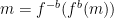
Slightly more secure might be to have Alice send $f^a(m)$ , have Bob not immediately decrypt, but instead compute $f^{b+a}(m)$ and send this back to Alice, and then have Alice compute $f^{-a}(f^{b+a}(m)) = f^b(m)$ . Now Bob decrypts the message by computing $m = f^{-b}(f^b(m))$ .

We can modify this further for use as a signature / authentication protocol: as a signature to Bob, Alice sends $f^a(f^b(w)) = f^{a+b}(w)$ to Bob; Bob computes $f^{-b}(f^{a+b}(w))$ and verifies that this matches with Alice’s public key $f^a(w)$ .

The security of these modified protocols are based on the difficulty of efficiently of deducing a and b or m, given only f and the images $f^a(m), f^b(m)$ and $f^{a+b}(m)$ ; i.e. the difficulty of the (analogue of the) discrete logarithm in generic infinite cyclic subgroups of the free group.

Questions: Do generic infinite-order automorphisms of the free group actually have good properties from the standpoint of these cryptographic applications? How much cancellation can we typically expect in freely reducing $m \cdot f^{a+b}(w)$ ? Moldenhauer’s arXiv preprint doesn’t appear to address these questions, although her thesis might.

Also: if Eve observes a lot of the Alice’s comunications secured using this last protocol, she will see a lot of pairs $(x, f^a(x))$ , since $f^{a+b}(m) = f^a(f^b(m))$ , and both $f^{a+b}(m)$ and $f^b(m)$ are exchanged in the protocol. How many of these would Eve need to collect before she can try to effectively reconstruct what $f^a$ is? How much will the cancellation / free reduction created by concatenating signatures (or other material) to the end of messages alleviate this?

Articles

Topology as squinting

One can describe topology, in more descriptive language, as the study of coarse-grained or qualitative features of space. Instead of asking about distances and angles, one asks about connectivity, compactness, the presence of holes (as captured e.g. by homology or more subtly by cohomology), the kinds of paths that live in the space (as captured by the fundamental group), and so on.

Sometimes this loss of precise information is desirable in applications: when we are inundated with data, a more coarse-grained or qualitative perspective can help us see the forest for the trees.

Below we describe two topological tools, both built off homology, which demonstrate this guiding philosophy and how it has turned out to be useful in certain applications.

Persistent homology

Homology is the topological tool of choice in many applications. It contains information about connectedness, compactness, and holes in all dimensions, is conceptually more straightforward than cohomology, and is eminently computable using the tools of linear algebra.

In applications we often start from a point cloud (i.e. a finite set of points) sampled from what we assume to be an underlying manifold. In order to reconstruct the homology of the underlying manifold, we could e.g. the nerve of an open covering constructed by taking balls based at every point in our point cloud, but are immedaitely faced with the question: how big should we make those balls / how fine a covering should we take? Persistent homology offers a compellingly natural answer to this question: use all possible scales, at once.

What is persistent homology?

Persistent homology, as described by one of its originators (Herbert Edelsbrunner), is “an algebraic tool for measuring topological features of shapes and functions [which] casts the multi-scale organization we frequently observe in nature into a mathematical formalism.”

The basic idea is to measure homology “at all possible scales”, and keep track of how homology varies as we pass between these various scales. Below we give more precise formulations of this for Morse functions, and then for triangulable spaces.

Given a Morse function $f: \mathbb{R} \to \mathbb{R}$ (i.e. f is smooth with non-degenerate critical points), we can consider the topology of the sublevelsets, and pair up critical points which cause connected component to be added or removed. A persistence diagram is a diagrammatic representation of this pairing (figure from Edelsbrunner-Harer):

persistd

We can generalize this idea to higher dimensions—for a Morse function $f: M \to \mathbb{R}$ on a n-manifold $M = M^n$ , we obtain n persistence diagrams, one in each degree $0, 1, \dots, n-1$ of (nonvanishing) homology.

Alternatively, we may define persistence homology on a simplicial complex (or more generally a triangulable space) K by specifying a filtration $\varnothing = K_0 \subset K_1 \subset \dots \subset K_m = K$ .

The work of Zomorodian and Carlsson, and many others following them, have fleshed out the theory of persistent homology considerably; the Edelsbrunner-Harer survey linked to above is a good starting reference. Some key results:

Persistent homology based on homology with k coefficients can be given a $k[t]$ -module structure;
Persistent homology is computable in a wide range of settings.
Persistence is stable under perturbations (the precise formulation here depends on the setting.)

Applications

One of the first applications of persistent homology was for shape recognition, via a generalization of convex hulls known as alpha shapes. Here we start with a point cloud, and would like to deduce the underlying shape from which (we assume) it was drawn. To do this we start forming alpha shapes—but as above there is a question of which scale we should use in this process. Persistent homology resolves this question by saying that we should take all possible scales, and regard features that “persist” across a (relatively) large(r) range of scales as more likely to be “true” features of the underlying shape.

The idea of persistent homology being potentially useful wherever homology might be useful, but questions of scale exist, can also be seen e.g. in its application to homological criteria for coverage in sensor networks. Given a network of sensors which can communicate with nearby ones, one can “detect” gaps in coverage as non-trivial elements of the second homology of a flag complex with 1-skeleton a sensor communication graph (vertices are sensors, and there is an edge between two vertices if the corresponding sensor ranges overlap.)

The formulation of such a criterion is almost tautological (“there is a hole if the algebra says there is a hole”), but one advantage it has is that second homology can be computed, in a distributed fashion, by the sensors in such a locally-communicating network—while we have not done anything significant conceptually, we have reformulated our intuition in a precise, computable way. To compute it in a robust, noise-proof way which does not require precise knowledge of distance between sensors, however, requires the use of persistent homology (or other tools.)

Topological data analysis

Persistent homology has also been a key tool in topological data analysis, starting with (I believe) the work of Gunnar Carlsson and Afra Zomorodian. The intuition there is that large data sets, while extrinsically huge-dimensional, are often intrinsically low-dimensional in nature, and topology, via persistent homology or other means, provides a good way of effective dimension reduction, because, very roughly speaking, “shape matters”.

The (statistical or other) theory to back this intuition is not always present, although at least on the mathematical side there has been considerable development, driven in large part by possible applications in topological data analysis, to put the theory of persistent homology and its application to data analysis on a sound mathematical footing. Stability theorems, in particular, show that persistent homology at least has a chance of being a sufficiently robust invariant to be useful in data analysis.

There have been a number of applications of these techniques, and indeed a start-up which has made topological data analysis its killer app, although the use of topological techniques in data analysis is still from systematic: successful applications often seem somewhat ad hoc; the generic attempt to apply topological data analysis seems more likely to result in a case of “I found these cycles in my data—but what does that mean?”

Euler calculus

An easier version of homology—or, really, a collapsed or “decategorified” version of it—is the Euler characteristic, and even with part of its topological power collapsed this can still serve useful functions.

For instance, one may notice that the Euler characteristic obeys something that looks like an inclusion-exclusion principle: $\chi(A \cup B) = \chi(A) + \chi(B) - \chi(A \cap B)$ . One can formalize this and build a theory of integration “with respect to Euler characteristic” ( $d\chi$ ) by defining $\int_A \chi_A \,d\chi = \chi(A)$ for characteristic functions of (sufficiently nice) sets, and then extending linearly and using limits.

The sense in which this is like a “squintier” version of Lebesgue integration (say) can be seen clearly in the axiom underlying that definition: instead of associating to the characteristic function $\chi_A$ of a set A the measure of A, we associate to $\chi_A$ the Euler charateristic of A.

The resulting theory is fairly nice—there is a Fubini theorem, Euler integrals can be efficiently computed via the Euler charateristics of level sets and related objects, &c. Not all functions can be integrated, but the ones that tend to be associated with finite point clouds can (a more precise formulation involves o-minimal structures; the functions which can be integrated are those with discrete range and definable preimages according to the o-minimal structure. The theory can be further extended to continuum-valued functions, but that introduces more technicalities, and we do not need it here.)

Schapira and Oleg first worked the theory out in the late 1980s, and by now it has found applications in tomography, sensor networks, and so on: we briefly describe a few of these below.

An application to tomography

The Schapira inversion formula is a topological version of the inversion formula for the Radon transform. Suppose we have a compact subset $T \subset \mathbb{R}^3$ , and we “scan” T by slicing along hyperplanes and recording the Euler characteristic of the slices of T—which, in the case of a compact set of the plane, is simply the number of connected components minus the number of holes (which equals the number of bounded connected components of the complement—a baby case of Alexander duality.) This yields a function $h: \mathrm{AGr}_2(\mathbb{R}^3) \to \mathbb{Z}$ (the domain here is the affine Grassmannian of all planes in $\mathbb{R}^3$ , not necessarily going through the origin.)

alexdual

Then we can recover the set T (via its characteristic function $\chi_T$ ) as follows: encode the information from the “scan” in the relation $\mathcal{S} \subset \mathbb{R}^3 \times \mathrm{AGr}_2(\mathbb{R}^3)$ by $(x,\pi) \in \mathcal{S}$ if $x \in \pi \cap T$ . We may verify h is related to $\chi_T$ by $h(\pi) = \int_{\mathbb{R}^3} \chi_T(x) \chi_{\mathcal{S}}(x,\pi) d\chi(x)$ (a Radon transform, but with $d\chi$ in the place of dx.)

Let $\mathcal{S}_x$ denote the fiber $\{\pi \in \mathrm{AGr}_2 (\mathbb{R}^3) : x \in T \cap \pi\}$ ; then $\chi(\mathcal{S}_x) = 1$ for all $x \in \mathbb{R}^3$ (each point in T appears on a compact set of affine planes) and $\chi(\mathcal{S}_x \cap \mathcal{S}_y) = 0$ for all $x \neq y \in \mathbb{R}^3$ (given $x, y \in T$ , the affine planes which see both of them are exactly the ones which contain the line containing both of them—and there is a circle’s—or technically a $\mathbb{P}^1$ ‘s—worth of such planes.)

The Schapira inversion formula in this case then states that we have $\chi_T(x) = \int_{\mathrm{AGr}_2(\mathbb{R}^3)} h(\pi) \chi_{\mathcal{S}}(x,\pi) d\chi(\pi)$ .

Thus in particular it is sufficient to record the connectivity data on the slices to recover the original shape, if one knows enough / has sufficient assumptions on the Euler characteristics of the slices. This seems almost too good to be true—until you realize that actually knowing the Euler characteristic for every slice is still a nontrivial problem. Still, it does give us some latitude to deform which was less present in the original, non-topological Radon transform.

An application to sensor coordination

Baryshnikov and Ghrist have applied Euler integration to the problem of target enumeration via distributed sensor networks. Here the setup is this: we have a bunch of enumeration targets (cats, perhaps, or something less fanciful, such as cars) in a space X covered by a sensor field (in actual applications to be approximated by a sufficiently dense network of sensors.)

Each sensor $\alpha$ records the total number of targets it senses in its range; the sensors can also communicate with nearby sensors (those with overlapping ranges) to exchange and compare target counts, but that is the limit of their capabilities. Given this, and that the sensor ranges overlap in undescribed ways, how should we go about recovering an accurate global count?

Let the target support $U_\alpha$ be the subset of all $x \in X$ s.t. the sensor at x senses $\alpha$ , and $h: X \to \mathbb{Z}$ is the counting function which simply returns the number of targets counted by the sensor at x. 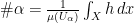In a toy case where $X = \mathbb{R}^2$ —so that we did not have to worry about boundary effects—and all the target supports were perfect circles of radius R, we would have $\int_X h \,dx = = \int (\sum_\alpha \chi_{U_\alpha}) = \pi R^2 (\#\alpha)$ , or $\#\alpha = \frac{1}{\mu(U_\alpha)} \int_X h\,dx$ , where here both dx and $\mu$ refer to Lebesgue measure.

Now, if all the target supports $U_\alpha$ have the same nonzero Euler characteristic N (e.g. if they are all contractible, so $N = 1$ ), then we can apply exactly the same logic, but using Euler integration instead of Lebesgue integration, to show that the number of $\#\alpha = \frac 1N \int_X h \,d\chi$ .

Hence we did not need our precise geometric hypotheses—that we had no boundary effects, and that all of our target supports were geometrically the same shape; we only needed looser, topological analogues of these hypotheses.

M	T	W	T	F	S	S
		1	2	3	4	5
6	7	8	9	10	11	12
13	14	15	16	17	18	19
20	21	22	23	24	25	26
27	28	29	30	31